07. Histogram in Action
Histograms in Action
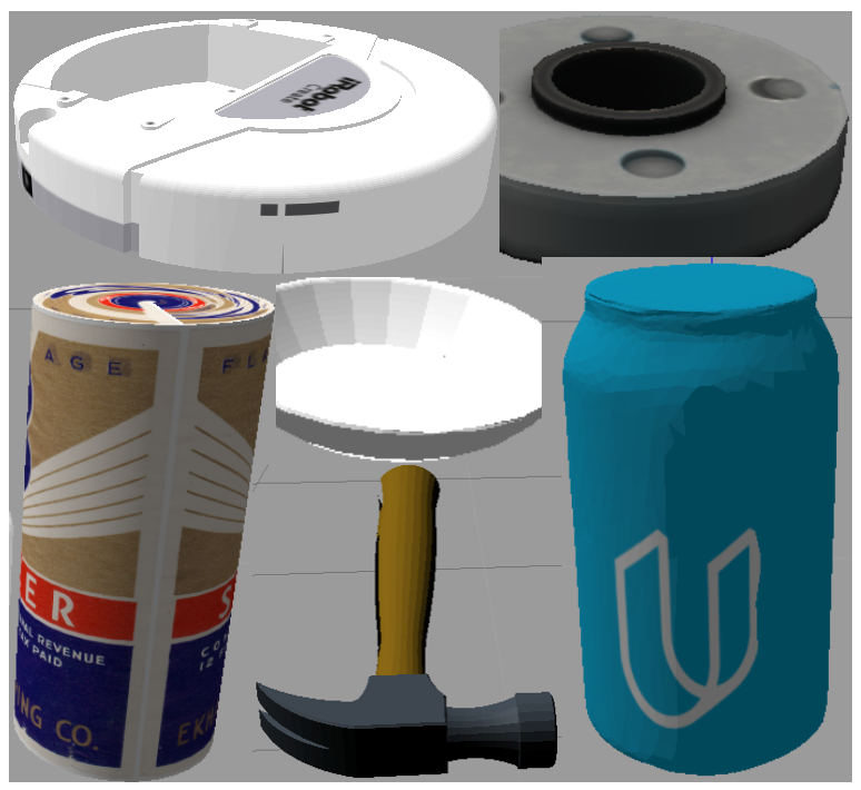
What do color histograms look like for these objects??
Using the point clouds that you generated, you will be asked to construct a color histogram for the points found in 3D space. However, for the purposes of an example exercise, operating on pixels in a 2D image will suffice. We will use the blue can as an example.
Here is the code to load our image:
import matplotlib.image as mpimg
import matplotlib.pyplot as plt
import numpy as np
%matplotlib inline

# Read in and plot the image
image = mpimg.imread('Udacican.jpeg')
plt.imshow(image)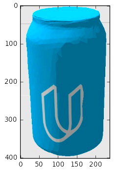
Now let's construct the histograms:
# Take histograms in R, G, and B
r_hist = np.histogram(image[:,:,0], bins=32, range=(0, 256))
g_hist = np.histogram(image[:,:,1], bins=32, range=(0, 256))
b_hist = np.histogram(image[:,:,2], bins=32, range=(0, 256))
With np.histogram(), you don't actually have to specify the number of bins or the range, but here I've arbitrarily chosen 32 bins and specified range=(0, 256) in order to get orderly bin sizes. np.histogram() returns a tuple of two arrays. In this case, for example, r_hist[0] contains the counts in each of the bins and r_hist[1] contains the bin edges (so it is one element longer than r_hist[0]).
To look at a plot of these results, we can compute the bin centers from the bin edges. Each of the histograms in this case have the same bins, so I'll just use the r_hist bin edges:
# Generating bin centers
bin_edges = r_hist[1]
bin_centers = (bin_edges[1:]  + bin_edges[0:len(bin_edges)-1])/2
And then plotting up the results in a bar chart:
# Plot a figure with all three bar charts
fig = plt.figure(figsize=(12,3))
plt.subplot(131)
plt.bar(bin_centers, r_hist[0])
plt.xlim(0, 256)
plt.title('R Histogram')
plt.subplot(132)
plt.bar(bin_centers, g_hist[0])
plt.xlim(0, 256)
plt.title('G Histogram')
plt.subplot(133)
plt.bar(bin_centers, b_hist[0])
plt.xlim(0, 256)
plt.title('B Histogram')
plt.show()
Which gives us this result:
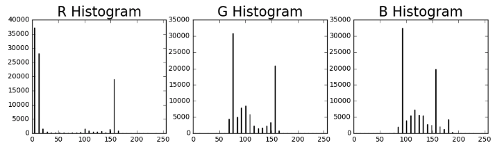
This plot now shows the RGB signature of the blue can! The feature vector associated with these histograms will then simply be the three distributions concatenated together like this (we'll also convert cast to float to ensure we don't do integer division in the next step):
hist_features = np.concatenate((r_hist[0], g_hist[0], b_hist[0])).astype(np.float64)However, to compare histograms of different total numbers of points, we'd like to normalize the result, which is to say, make it such that the sum of all the bins in the histogram is equal to 1. A simple way to normalize is by dividing by the sum of the entire histogram:
norm_features = hist_features / np.sum(hist_features)In addition, it can be advantageous to construct this histogram in a different color space. In the exercise below, your task is to first convert the RGB image to HSV using the cv2.cvtColor() function, then construct a normalized histogram of the converted image.
Having a function that does all these steps might be useful for the project, so for this next exercise your goal is to write a function that takes an image and computes the normalized HSV color histogram of features given a particular number of bins and pixels intensity range, and returns the concatenated feature vector, like this:
```python
Define a function to compute color histogram features
def color_hist(img, nbins=32, bins_range=(0, 256)):
# Convert from RGB to HSV using cv2.cvtColor()
# Compute the histogram of the HSV channels separately
# Concatenate the histograms into a single feature vector
# Normalize the result
# Return the feature vector
```
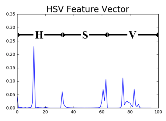
Your output should look similar to this, where the x-axis corresponds to histogram bins and the y-axis corresponds to what fraction of the signal comes from each bin. This is now the HSV color signature of the image, where the first 32 bins along the x-axis (left side) correspond to the H-channel, the next 32 (center) to the S-channel and the last 32 (right side) to the V-channel.
Start Quiz: